
This paper describes two determinant aspects in the technological development of machines and production systems: the evolution of quality control systems from “passive” aimed at the rejection of nonconforming product to “active” systems for process management and optimization and the advent of artificial intelligence and “machine learning” in process control. We will demonstrate certain technical aspects and the relative experiments in machinery and production systems.
The drawn bar market represents a pillar of the mechanical production chain on a worldwide level. The last ten years has witnessed significant pressure on the production sector crushed between the higher demand for quality and higher demand for less expensive products. Thus a growing need has been created for production systems and technologies that quickly meet this precise request of the sector. As in many other production technological fields it was suddenly faced with the complexity of having to reconcile a medium-slow development pace of technologies and production organizations with a rapid evolution in the demand for finished product quality and certification. This paper will explore some of the automation logic of systems and machines normally used in manufacturing drawn products, the relative main aspects of process control and the respective architectures, the quality control systems mostly involved in these development processes, some introductory aspects on artificial intelligence techniques and developed control technologies, experiments and achieved results, applications in machines manufactured with these emerging technologies and future prospects.
Automation processes and relative architectures
Industrial production systems have a distributed architectural control structure that is now consolidated and structured on 4 levels:
Level 0: “the field”, i.e. the mechanical and power part of the system, where the production process is actually
created.
Level 1: “direct control”, i.e. the direct automation part that supervises the management of the automations
necessary for carrying out the production process.
Level 2: “supervision”, i.e. the configuration management part of the control systems and
production schemes.
Level 3: “advanced control and saving historical data”, i.e. medium-long period memorization of the data from
level 2 in order to generate mainly off-line optimization strategies of the configurations.
Level 4: “management level”, i.e. the centralization and statistical summary of saved historical data in order to permit MES (Manufacturing Execution System) and ERP (Enterprise Resource Planning) activities.
Specifically, the implementation of MES systems, even if in the form of a basic service, was the backbone of the first season of development and dissemination and called “Industry 4.0”. Our work starts from the consideration that the control system of a machine or a system is composed by a network of distributed processing devices which basically include three fundamental interfaces: 1) interfacing towards the physical product realization Process; 2) interfacing towards the operator for line management; 3) interfacing towards the managerial structure.Thus the production system control loops are identified on three levels: the first “direct” in the management of the system mechanisms (level 0 managed by level 1) the second for the “operator” which entails the regulations necessary in order to keep the product within the specifications requested by the customer and market (HMI access through level 2) and the third for “management” which handles monitoring and correcting the system use strategies based on the production efficiency goals for the expected profit.
The drawn product manufacturing process
The production architecture we are referring to is composed of a processing process from roll to bar where the salient product elements basically refer to the geometric characteristics of the part such as the straightness, geometric regularity, finish and the quality of the bar facing processing.
Process from roll to bar
This type of processing is normally divided into: prestraightening, drawing, straightening, cutting, finishing of the ends and packaging. One of the weak aspects of current systems is composed of the process control loop referred to the realized quality; this is a loop that passes through operator supervision methods based on the information produced by the quality control systems; basically the product quality and its constancy are mainly managed by the operator’s expertise and synthesis of the production settings based on previous experiences related to factors that cause the obtained characteristics to deviate in relation to the factors around the production process.
Artificial intelligence, Machine Learning and Fuzzy Cluster Analysis
Our work entailed the application of artificial intelligence, machine learning and fuzzy cluster analysis technologies to build an automatic system in the process control loop referred to the quality result. The system analysis procedure that we are illustrating is organized in a two phase process: the first based on a statistical analysis at the end of the monitoring cycle and the second based on clustering of the cycle just analyzed with those accumulated during production process management. The first level consists in the mathematical analysis of the cycle just completed in the observation window through the construction of a structured statistical synthesis. The monitoring window parameters are essentially tied to the change in the main characteristics of the processed product or at the end of the production batch.
The selection of these analytical window conditions is primarily connected to machine technical parameters such as the operating temperatures of processing tools since based on our experience we have found for example that when a machine is left off even for just a few minutes variations of the operating conditions can be created comparable at times to variation of the processed material characteristics. When the end of monitoring cycle conditions are reached, the statistical analysis phase of the cycle itself starts. This process includes the previous definition of a set of standardization parameters which can describe the type of phenomenon implied in the control cycle with sufficient precision i.e. the set of parameters must be adequate for correctly defining the cycle type based on the aims set for the control. For this analysis concept we decided to use two mathematical structures; the first is the set of statistical parameters that we have called “GENES” and the second is the vector of these parameters that we have called “DNA”; a “DNA” with its “GENES” thus represents a good representative photograph of the process behavior in the considered analysis window.
In this manner the DNA represents the standardization and the GENES constitute the set of characteristics that characterizes it.
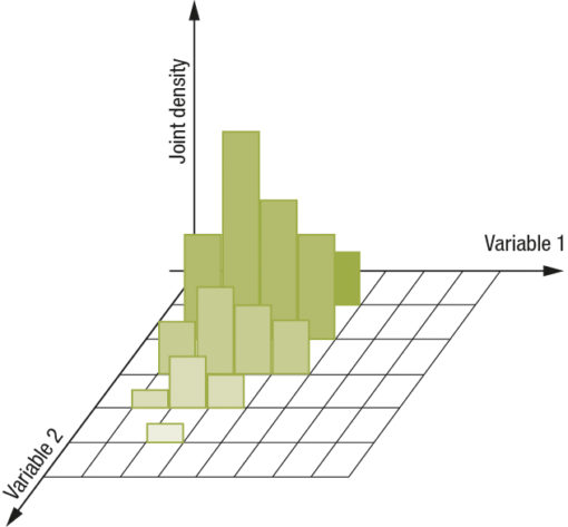
The GENES we use are basically statistical parameters because they maintain the information necessary losing the temporal extension. There are three types of GENES:
- Joint distributions
- Single dimension distributions
- Scalar
Solutions with multi-dimensional distributions were excluded from the selection of GENE type since they require excessive memory use, with an exponential type trend. Thus by limiting the number of dimensions, but structuring an opportune DNA, we are nevertheless able to maintain a significant amount of information. The result in this case is that the DNAs represent points in a hyperspace and the GENES represent dimensional variables that unequivocally identify the position in a DNA in the same hyperspace.
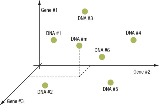
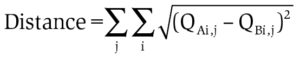
Fig. 1 Space in case R3
This approach makes it possible to construct sets of process physical parameters that can be later correlated to reference values that are subject to control, i.e. to the requested quality parameters. Basically, parameters like the input material characteristics and setting parameters of the production system create a structure of information that will thus be correlated to the final result. The second part of the algorithm entails the recognitionof the “similarity” of what was just observed compared to the previous observations memorized inthe historic data referred to the desired quality results. This phase starts at the end of the observation time window. When a cycle ends, the system essentially possesses the DNA of what just happened, and can compare it with the DNAs of previous cycles in order to assess their differences. The collection of memorized DNAs thus represent a kind of collection of cycle types based on the difference of GENES inside the DNAs; this mathematical structure makes it possible to perform these analyses in geometric form inside a space where the DNA is a point and the GENES represent the coordinates that define its position in the hyperspace.
Basically we work in a non-Euclidean space where the dimensions are not uniform by type since they are composed of multi-dimensional statistical distributions.
In Fig. 1 a simplified case is shown where the DNA is composed of a vector of 3 GENES and the GENES are scalar statistical information. This vision of the analysis space is a simplified vision, but it is correct; it is possible to think of something similar even in the case where some genes are actually statistical distributions even with two or more dimensions.
This simplified vision is rigorous to the extent where we can still define a concept of distance. To do this we use part of the theorem of χ2 according to which the distance between two single dimension distributions may be given the following values: Fig.2
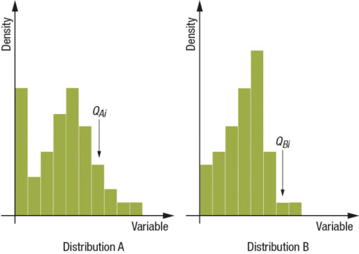
Supposing: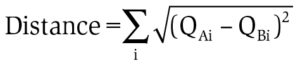
we obtain a definition of distance between the two standardized distributions. In the case of joint distributions this principle remains valid by defining a path inside the matrix so that it is always possible to extract a one dimension distribution from a two dimension distribution where it is possible to apply the definition just stated; what I obtain is the following situation: Fig.3
In this case the notion of distance between two joint distributions, if i is the index for a variable and j is the index for another variable, assumes the following definition:
The situation we find ourselves in at the end of a cycle is roughly the following:
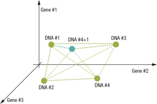
Fig.4
Based on the distances between all the possible cluster pairs a decision is made which will be the two clusters to join; this decision is made based on a calculation of the barycenter value, i.e. through a weighted average that takes into account the weight associated to the two clusters. The radius of the new cluster in question is also updated based on the distance. For example, this is what could happen if the DNAs of the previous example had the following weights Fig.5 e 6
In the example we see how the new DNA just found is compared with the previously memorized ones in order to understand if what was just found is a new standardization or if it represents an already known standardization. Over time the centers will stabilize in space and will thus be correlated to the requested quality benchmark parameters. This historic memory, synthesized and reorganized at every cycle, constitutes what the control system has learned regarding the final result in relation to the operating conditions thus to be able to act as the basis for the production process active control strategy.
Industrial application
We have applied this algorithmic method in a drawin process of a circular cross-section product.
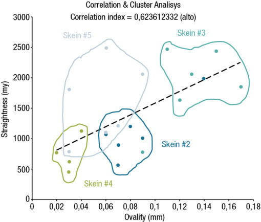
The DNAs were set with specific GENES referred to metal processing information such as the dimension of the crystalline grain, morphological type information such as the ovality of the round bar and process information such as the line speed and product deformation cycle settings compared to the final straightness result.
Over time recurring standardizations clustered thus making it possible to identify and adjust the process in order to maintain a quality level in line with the expected reference values. Micrograph referred to material with excellent straightness characteristics. Micrograph referred to material with poor straightness characteristics.
Conclusions
This mathematical approach provides a valid method for building a system that automatically learns from the occurrence of recurring situations correlated to the desired result in order to accumulate a type of clustered historic data to act as a setting parameter of the process itself. Basically it becomes a control system with the ability to recognize situations that have already occurred in order to implement the best operating strategies. In conclusion, this represents a learning method that makes the control system expert through an automatic learning mechanism.
The authors

Mauro Stefanoni is the managing director of SAS Engineering and Planning Srl and the co-founder and co-CEO of Aequilibrium Srl. He is mechanical engineer and business owner with many years of experience in the design and manufacture of machines for the production of cold drawn products.

Gabriele Bomba is the co-founder and co-CEO of Aequilibrium Srl. He is a mechanical engineer, business owner, and expert in the analysis and modeling of mechanical systems, development and application of artificial intelligence in control systems, and the application of machine learning in optimization processes. He is the author of several innovations in the field of straightness measurement of lean products.
References
[1] Fuzzy Cluster Analysis – Frank Hoppner, Frank Klawonn – Rudolf Kruse – Thomas Runkler – Willey
[2] Knowledge-Based Clustering – Witold Pedryez – Willey
[3] Modern Control Engineering- Katsuhiko Ogata – Prentice Hall
[4] Simulation of Dynamic Systems – Harold Klee –CRC Press


